John Murphy's Patterns in a nut shell

     These are the rules compiled from the text,  Technical Analysis Of The Financial Markets by John Murphy. I have taken pains to compile these rules, for my own personal use. But I have also published it so that, others can gain from it. It is most recommended to read the full text by John Murphy before going through this material.

All the figures are edited and used from the book-Technical Analysis Of The Financial Markets by John Murphy

TRENDLINES

1. Wait for the prices to close 3% below the trendline, to confirm a trendline breach.

2. Along with rule 1, wait for the prices to close below the trendline for atleast two consecutive days, to confirm a breach of the trendline.

3. While using trendline fans, the third line breach is considered to be a valid trend reversal.

3. After the breach, the price of a security generally tend to move upto the same distance in the opposite direction of the trend, as the last top or bottom. If a channel is present, then the width of the channel is the distance upto which, the prices will move, once the basic trendline is breached.

5. Most important and healthy trend lines follows a slope of 45°. If there are steeper lines, they might finally be breached and corrected to a 45° trend line. And if there is a shallow trendline, the trend might either be not valid or will gather steepness over time.

6. Even if there is a trend, a channel may not exist.

RETRACEMENT

1. The retracement levels according to dow theory are 33%, 50% and 66%.

2. The retracement levels from the dow theory can be combined with Fibonacci retracements of 

38.2%, 50%, 61.8% to form ranges of retracements as 33-39% and 62-66%.

REVERSALS

1. A reversal happens when  a new top is reached in an uptrend, but the prices finally close below the previous close. Or, when a new bottom is reached in a downtrend, but the prices closes above the previous close.

2. This can happen in any time frame, but when the price reversal happens on fridays in a weekly time frame, or on month ends in  a monthly time frame, then the significance increases.

3. On the reversals if volume is is especially high, then it might indicate a trend reversal or atleast an intermediate correction.

GAPS

1. Weekly and monthly gaps are very significant, but occur rarely. Some gaps are filled and some are not. The three types of gaps given below, when satisfied with certain other conditions, are most likely not filled.

BREAKAWAY GAP

       

2. A break away gap occurs after an important price pattern is completed ( like Head and Shoulders ) and the resistance is finally broken or, when a major trend line is broken due to a trend reversal.

3.  If accompanied by heavy volume, break away gaps are most likely not filled. 

4. Break away gaps form a significant trend support, the trend which the gap already started. 

5. A close below the Breakaway gap, while in an uptrend, usually signifies weakness and a trend reversal.

RUNAWAY OR MEASURING GAP

6. A measuring gap occurs almost in the middle of a trend. It confirms the smooth continuation of the trend.

7. Measuring gap also acts as supports and are most likely not filled. And if at all, when filled, can signify a trend reversal.

EXHAUSTION GAP

8. This occurs as a last gasp, at the end of the trend.

9. It is confirmed, when the prices finally closes below the gap after a few days or weeks of the occurrence. 

10. Once the gap level is broken, a significant trend reversal can be expected.

11. Sometimes the gap level is broken with another breakaway gap, in the opposite direction. As a result, the price movement between the exhaustion gap and the subsequent break away gap looks like an island. When an island reversal happens, a trend shift can be expected.

Note that the island formed on the top usually contains more than one price bar ( In the figure above, there is only one price bar in the island area )

REVERSAL PATTERNS

    The price picture patterns are used to predict what happens, after a trendline is broken and the market moves side ways; whether the market moves sideways or the trend reverses.

GENERAL RULES

1. The major reversal patterns are Head and Shoulders, Double/Triple tops and bottoms, V (spike) tops and bottoms and Rounding (saucer) patterns.

2. The major continuation patterns are triangles, flags, pennants, wedges and rectangles.

3. Volume levels are used in confirming the indications of these patterns.

4. These patterns can also be used to measure the extent of the subsequent movements.

5. A prior trend should exist as a prerequisite.

6. A major trendline needs to be broken before the pattern manifests.

7. Larger the pattern, the more significant it becomes, and greater the subsequent price movement.

8. Topping patterns are shorter, more volatile and fast forming while bottoming patterns takes time to form and are less volatile. 

9. Therefore, though bottoming patterns are less risky, topping patterns are more rewarding, as prices falls faster than they build up.

10. Sometimes, the breaking of a major trendline coincides with the completion of a price pattern.

11. The completion of price pattern should accompany an increase in volume, especially in bottoms.

12. If volume do not increase during an upside break out, then the pattern cannot be trusted.

HEAD AND SHOULDERS PATTERN

1. Most of the other reversal patterns are a variation of H & S pattern.

2. Volume expands on reaching each new crests, and contracts on each new troughs, before the pattern starts to form ( before the trend loses steam ).

3. When the left shoulder starts to form, the volume may get lighter than the previous crests. This is an indication that the trend is losing steam, and a pattern formation can be anticipated.

4. When trend line is broken, there is a possibility of a H&S formation. Volumes get increasingly lighter on crests and increasingly heavier on subsequent troughs.

5. Formation of point E below the highest peak of point C, is when the trader starts to prepare for a position. When this happens, its almost sure that a sideways movement has started, and liquidation of long positions may be wiser. By this time a Neck line can be drawn.

Neckline and Subsequent actions.

a) The H&S pattern is confirmed when the neckline is broken.

b) Neck line is the new trendline, drawn after the sideways movement starts. A return move on lighter volume with peak at point G can be expected if the neckline is broken with not so heavy volume. If the neck line is broken with very heavy volumes, a return move may not be there or a small return may occur.

c) Either a 1-3% close below the neckline or two successive closes below the neckline, has to be used as a criteria for the H&S formation confirmation. Other wise, resumption of the uptrend can happen.

d) Though volume can be lighter in the second peak ( Head part ) it has to be lighter on the third peak ( Right shoulder ). The volume should be heavier while the breaking of the neck line, and should be lighter again on the return move, and should increase again, on the subsequent downward move. The volume has to pick up at some point in the down trends, AT THE LEAST.

e) Since neck line is a sideways trend, the minimum target for profit booking, is always the width of the trend, in this case, the height of the head from the neckline. ie, the prices are most likely to move below the neckline, the same distance as the height of the head from the neck line. Maximum target depends upon the support levels, retracement levels etc. Minimum price target should also be adjusted to price support levels.

f) The slope of the neck line is slightly upward in case of a top H & S and slightly downward in case of an inverse H& S. However exceptions do occur. 

Inverse H & S pattern

a) The main difference between the topping and bottoming pattern is volume. A reversal from any downtrend happens only when there is absolute demand. The markets should trade on very heavy volumes when the trend reversal happens, when new peaks are reached, especially when the neck line is breached. Whereas, the market prices may fall on inertia alone ( lack of demand or direction ) on market tops. The volume is absolutely critical on reversal on inverse H & S. If not, it is risky to take trades on bottom reversals.

b) The resulting new uptrend should also be on heavier volumes.

c) There is a greater tendency for a return move.

Complex H&S Patterns

a) There might some times be a formation of a double head, or double shoulders.

b) If double left shoulders are present, then double right shoulders also have to be present.

TRIPLE TOPS AND BOTTOMS

1. These are actually a slight variation of H&S pattern and are rarer.

2. All the rules for head and shoulders pattern should be followed.

DOUBLE TOPS AN BOTTOMS

1. This kind of pattern follows the same rules as the H& S pattern except those mentioned below.

2.  Point B price level acts as the neckline here. The breaking of this line accompanied by heavy volume confirms the pattern.

3. There is no right shoulder for this pattern, and therefore, after the second peak (The head as in H&S) is formed, and when the neckline is broken ( Point B support), the pattern is completed.

False Double Tops

In order to avoid false double tops the following rules needs to be followed

a) In an uptrend or down trend, sometimes, consequent peaks or troughs may be of the same level, which is quite normal as shown in the fig below

b) Volume pattern should be exactly followed as of H&S pattern.

c) The neckline has to be broken with higher volume, to confirm the pattern as shown in the figure below.

d) The More the gap between the two peaks, the more probable for the reversal.

e) Some times, a close of 1-3% above the first peak level, or a two consecutive close,  are used to filter out the false break outs. But Volume pattern will filter out most of the false break outs.

SAUCER

1. They are slow and gradual in forming.

2. They might span several years. It is difficult to predit how long it takes to form the pattern or how far the prices will move in the opposite direction.

3.  The longer it takes, the more significant it becomes.

SPIKES

1.  They happen, when the market gets over extended and a sudden adverse news cause the prices to fall very abruptly.

2. A daily or weekly reversal accompanied by heavy volume is sometimes the only warning.

ASCENDING AND DESCENDING TRIANGLES AS TREND REVERSAL PATTERNS

Please look at the end of the descending triangles discussion.

WEDGE REVERSAL PATTERN

Please look at the end of the Wedge pattern discussion.

CONTINUATION PATTERNS

GENERAL RULES

1. Continuation patterns are usually formed in short or intermediate time duration.

2. Sometimes, some of the continuation patterns can act as reversal patterns in special cases.

3. Volume should diminish along the progress of the pattern.

4. Please read also, the H&S pattern rules carefully 

TRIANGLES

1.  Triangles are usually intermediate patterns, but some times occur in long duration, which are much more significant.

2. Minimum requirement of a triangle is 4 reversal points, but sometimes triangles with six reversal points can also be seen.

3. The prices must break out between two thirds to three forth, the length of the triangle. If the prices do not break out even after three forth of the length of the triangle then the triangle has lost significance.

4. A return move can be expected towards the broken line.

5. A broken line reverses its rule after the break out. ie in an uptrend, the resistance line ( the upper line ) is broken. But after the break out, the upper line becomes the support line.

6. Diminishing volume rule applies.

7. As in the reversal patterns, to confirm an uptrend continuity, the volume should be more in upward movements within the triangles. This is more significant in uptrend confirmations than down trend confirmations.

Symmetrical Triangle

1. Referring to the fig above, only after fixing the fourth point, the symmetrical triangle formation can be confirmed.

2. The two third to three forth break out rule applies here.

3.  Diminishing volume rule applies.

4. Rule 7 for the Triangles to be followed.

5. To measure the movement, draw a trend line as shown in the fig below, then follow the channel measurement rule. Please read also, the H&S pattern rules carefully.

Ascending Triangle

1. This pattern indicates there are more strength in buyers than sellers. And is generally considered as as a bullish pattern.

2. It works as a consolidation, and a trend confirming pattern in a bullish trend.

3. Break out move normally happens with heavy volume, return move with light volume can be expected.

4. The minimum target distance after the break out can be taken as the width of the triangle base.

5. Diminishing volume rule applies. But the strength of the volume should be slightly tilted towards the upward movements. Please read also, the H&S pattern rules carefully.

6. These triangles are more of an intermediate pattern, with long terms, rare. Short term formations are called Pennants, which are discussed shortly.

Descending Triangle

Descending triangle follows the exact same rule as that of the ascending triangle as it is a mirror image of the ascending triangle.

Ascending and Descending Triangles as trend reversing patterns.

1. Both ascending and descending triangles sometimes appears as topping and bottoming patterns. 

2. If an ascending triangle appears at the end of a down trend, and if a break out happens, then a trend change can happen. Same for the descending triangles which appear at market tops. Remembering rule 7 for triangles helps.

BROADENING FORMATION

1. This is a relatively rare pattern.

2. The volume tends to increase along the formation of the pattern.

3. This situation signals a market which is out of control.

4. It occurs when public participation is very high, especially at major market tops. It normally occurs at the end of major bull markets and is a bearish pattern.

FLAGS AND PENNANTS

1. Flags and pennants are quite common, are similar in appearances, occur at about the same place in an existing trend, and have same characteristics.

2. They occur when market pauses briefly to catch breath after a steep move with heavy volume. when they are at the process of formation, the volume declines, then again bursts on a break out.

3. They rarely produce a trend reversal.

4. Flag is a parallelogram with a slop against the slope of the trend. 

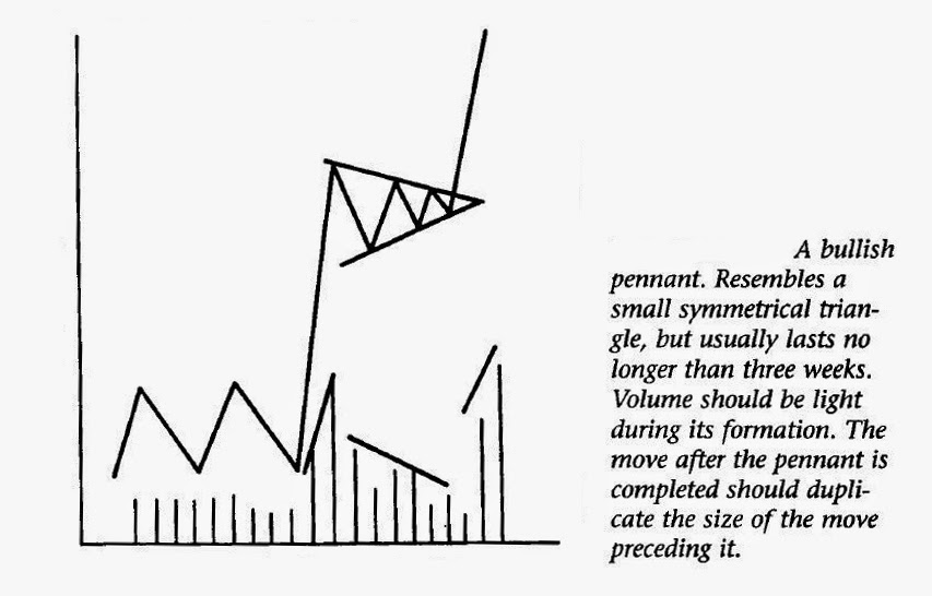
5.  Pennant is a small symmetrical triangle.

6. The volume should decrease along the formation of the pattern. and the break out should be with heavier volume.

7. They take shorter time to form usually two to three weeks, down trend patterns are shorter in duration.

8. Both the patterns are formed in the mid point of a market trend.

WEDGE PATTERN

1.  Wedge pattern follows all the rules of the triangle pattern, except its implications and rules cited below. Please read also, the H&S pattern rules carefully.

2. The wedge pattern has a noticeable slant.

3. A down ward slopping wedge is a bullish pattern, and vice versa.

WEDGE REVERSAL PATTERN

Since a falling wedge is a bullish pattern, when it occurs at the end of a bear market, it might signal a trend reversal and vice versa.

RECTANGLE PATTERN

1. Rectangle is a trading range, a congestion area.

2. Rectangle pattern with 6 price swings, can be misinterpreted as a triple top reversal. Triple top reversal volume rules needs to be checked and the pattern ruled out, before confirming a rectangular pattern. Normally the rectangular patter resolves towards the trend direction. However, the direction of the heavier volume side determines to which side the rectangle break out finally will happen.

3. Minimum target rule follows the channel minimum target rules. Please read also, the H&S pattern rules carefully.

CONTINUATION HEAD AND SHOULDERS PATTERN

1. The continuation H& S pattern forms inverted to the reversal version in a continuing trends.

2. However the rules follow that of the rectangle formation.

Current Account Deficit Vs Fiscal Deficit, a simple explanation

I am starting with an extremely simple definition for the two.

Current Account Deficit

          It is the difference between the total exports and imports of the country. Current Account Deficit in a period happens when the imports in dollars crosses the exports for a country.

Fiscal Deficit 

          It is the difference between the total revenue ( Mainly from taxes ) of a country and the total expenditure ( Mainly public expenditures ) of a country. Fiscal deficit in a period happens when the expenditures crosses the revenue.

Why profit is the highest when marginal cost curve crosses the marginal revenue curve ( Competitive firm model )

     The definitions and the characteristics for the various terms need to be referred to a standard text book. 

This blog will discuss only the reason for why the profit is maximized when Marginal cost curve crosses the Marginal revenue curve.

Abbrevations

MC=    Marginal Cost                                                     MR=   Marginal Revenue

ATC=  Average Total Costs                                           TC=     Total Costs

AVC=  Average Variable Costs                                     TR=     Total Revenue

AFC=  Average Fixed Costs                                          P=        Price; Q=    Quantity

Consider the following example

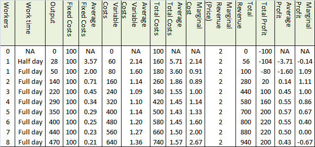
The table below gives the details of a factory producing a certain unit of a product.

Table 1

It is mentioned in a previous blog, why marginal cost crosses the Average cost curves at their lowest points,  and how the marginal cost, which is a change in cost, actually affects all the average costs.

EXPLANATION

Consider the following plots, plot 1 and plot 2 derived from the factory data in table 1.

Plot 1

Plot 2

The Total Cost is equal to Average Total Cost  multiplied by the quantity, and Total Revenue is equal to Average Total Revenue ( equal to price or MR for a competitive firm) multiplied by the quantity. Total Profit is the difference between the two.

In Plot 2, Total cost is drawn as an area which is equal to ATC multiplied by Quantity. And Total Revenue is drawn as an area which is equal to ATR multiplied by Quantity. Total profit is the Total Revenue area minus the Total cost area.

For example.

For a Quantity H, the TC=     area EYHF

                                 TR=      area DIHF

                                 Profit=  area DIYE.

For a Quantity G, the TC=     area ABGF

                                 TR=     area DCGF

                                 Loss=  area ABCD

CONFUSION

1.       In theory the profit has to be highest at a production output where the marginal cost crosses the marginal revenue, which is at point Z. whereas, it can be clearly seen that the Average total cost is lowest at point Y. And also, marginal cost is lower at point Y, which is lower than at point Z.

2.       At point W, the marginal cost is the lowest, much lower than the marginal revenue. But the production is at a significant loss at the same point.

CLEARING CONFUSION 1

Consider the following plots 3 and 4. Plot 3 plots the Total Revenue and Total costs. And plot 4, plots the difference of Total cost and Total Revenue ie the profit.

Plot 3

Plot 4

From plot 4 it is quite obvious that the maximum profit occurs at point Z ( where the MC crosses the MR). It is also observable from plot 3.

REASON    

The reason for this confusion is that, MC as defined previously is a change in cost. The difference between AVR( the straight line of $2) and the ATC curve gives us Average total profit(AVP), and it is quite clear that AVP is the highest at the point Y where ATC is the lowest. We get confused because we think that the profit should be highest when the AVP is the highest. But AVP is only an average. Increasing the production from point Y to point Z definitely reduces the AVP. But it increases the total profits. AVP is reduced because, each quantity  produced after point Y yeilds lesser profits, bringing down the average. But  the total profit gets increased albeit with decreased rate. Even when the Average Total Cost is at its lowest when the production reaches point Y (370 units), we can still squeeze in more profit per unit, by producing until the production reaches point Z (440 units) . Until then, each change in cost/ unit (MC) is still less than the price for which those units can be sold. The increase in total profits becomes zero only when the production reaches point Z. This is quite clear in the Plot 5.

 The difference between MR and MC is called Marginal profit, whereas, the difference between ATR and ATC is Average profit. In order to maximize the Total profit, we have to go on producing until the marginal profit is diminished to zero. Since Average profit is just an average, it might be still be positive for many more units of production even after the production crosses point Z. For more clarity refer to plot 5.

                                                                             Plot 5

In Plot 5, we can see that the average profit is maximum at point Y, which is self explanatory.

CLEARING CONFUSION 2

Marginal Cost, Marginal Revenue and Marginal Profit  are also the slopes of the Total Cost, Total Revenue and the Total profit curves respectively.

So in this case, when Marginal Cost is at the lowest, the Marginal Profit is at the maximum. But the factory is in loss. It just says that the slope of the Total cost curve is at the lowest and is about to change, and the slope of the Total profit curve is at the maximum and is about to change. At this point the Total cost is not the lowest, neither is the Total profit the highest. This is amply demonstrated in the plots 3,4 and 5.

Why the diminishing marginal utility curve has the same slope as the demand curve

Diminishing marginal utility states that, the marginal utility of a product diminishes with each unit of the product consumed.

This is because, the change in utility, when each unit of product is consumed, always decreases. ( refer to a standard text for more clarity)

ILLUSTRATION

Fig 1

Consider an example of ordering pizza, which costs one dollar a slice. If consuming the first slice gives 24 utils of utility, after eating the next one, the total utils increases to 36 utils. Refer to fig 1 for the complete pizza consumption.

You may notice that, had the price of a slice of pizza been $2, then the utility also reduces by half for each slice.

Fig 2

If we draw the total utility against number of slices consumed, the plot will look like fig 2

And therefore, if you plot the marginal utility in y axis and the number of unit consumed, in the x axis, you always get a curve with diminishing curve. This is called the diminishing marginal utility curve as illustrated in the fig 3 below.

Fig 3

If marginal utility of a product  is Mx at a price x, then Mx/x ie the marginal utility per dollar for that product should always be greater than that of any other alternative product, so that you may keep buying it.

So some one has to make you buy the same product  again and again, over every other alternative products, then the ratio Mx/x needs to be made constant, every time you consume the product.

Since marginal utility keeps on decreasing, while we consume the same product again and again, Mx decreases when more quantity is bought.

So inorder to keep Mx/x constant, the only way to do is the decrease the price, in the same ratio of decrease in Mx.

So the greater the price reduction, the more you will consume or demand. This is why the demand curve has the same slope as the marginal utility curve.

The demand curve is a plot produced, when the demand ( measured in quantity ) is plotted in x axis and the price plotted in the y axis.

The demand curve also has negative slope, ie the demand always diminishes when price is increased, keeping all other factors constant.

In the above pizza example, the demand curve would look like this

ILLUSTRATION

Product 1

let the marginal utility for a product be 100, 80, 60, 40, 20 for the first 5 pieces, and the price for the fifth piece is 20, then Mx/x for fifth piece is 1.

Product 2

If the marginal utility for another product be 100, 90, 70, 50, 40, and the price of the fifth piece is 20, then Mx/x for the fifth piece is 2.

If the seller has to make you take the fifth piece of the first product over that of the second product, then the marginal utility per dollar of the first product should be more than 2 ( marginal utility per dollar of the second product) . Ie the price of the fifth piece of the first product has to be reduced below 10 in order to make you buy the fifth piece of the first product over that of the second product.

This means that whenever you increase a price of a product, the demand diminishes.

Why Marginal cost curve crosses the Average Total Cost curve and the Average Variable Cost curve at their minimum point.

Refer to figure 1 given below.

                                                                        fig 1

All the data is taken from the chart in the blog on "Why the profit is maximised when the marginal cost curve crosses the marginal revenue curve"

Facts to consider

1. Average total cost curve is a plot of the average total costs for all the different quantities starting from zero production. The X axis is the quantity, and the Y axis is the ATC. This curve first slopes downward, then reaches a bottom and then slopes upward.

2. Average variable cost curve has the same characteristics of the ATC curve, but always stays below the ATC curve at all the points. The difference between the values of the curves is the fixed cost.

3. Since all the three curves has quantity in the x axis, all of them can be drawn together. The MC curve also first slopes downward, reaches a bottom and then starts sloping upward. The MC curve first crosses the AVC curve and then the ATC curve at their respective bottoms. Refer to a standard text on the problem.

TC       :                   Total cost
dTC     :                  Change in total cost
VC      :                   Variable cost
ATC    :                  Average total cost; AC is the average cost
dATC  :                  Change in ATC
AVC   :                  Average variable cost; VC is the variable cost
dAVC :                   Change in AVC
FC      :                   Fixed Cost.
Q        :                  Quantity.
dQ      :                  Change in Quantity.
MC     :                  Marginal cost.

MC    =                 dTC/dQ
TC     =                  VC + FC
dTC   =                  dVC+dFC

But since FC is the fixed cost and by definition does not change, dFC = 0

So dTC=dVC

So MC = dVC/dQ

            This means that marginal cost, which is the change in total cost per unit of quantity is actualy caused by the change in variable cost only. Now here the question is why the marginal cost curve crosses the Average total cost curve and the Average variable cost curve at their respective bottoms.

             Consider the average of height in a class. Whenever a new student joins, the average changes. If the height of the new student is the same as the present average, then the average does not change, if it is less the average decreases, if it is more the average increases. 

           
             Similarly, the marginal cost is the next new comer. Marginal cost is the next change in the cost (per unit). This next change, if it is more than the average, then the average will increase or vice versa.

             Since MC = dTC/dQ = dVC/ dQ. The new comer is same for both the averages TC and VC.

So, both the AVC and the ATC curve decreases and increases due to the new comer entry MC.

            Now, in the portion of the curves, where they have a downward slope, before they hit their bottoms, the marginal cost values are lesser than than the respective values of the average curves. So the lower MC values drags the averages down. Now when the MC curve, which hits the bottom of its own, slopes upward and first crosses the AVC curve. At the crossing point MC value = AVC value. And after that the MC values drags the AVC curve upwards. This is also what happens to the ATC curve.

            Note that MC is the new comer for both the the averages as we proved earlier.

 

TAX ASSETS, LIABILITIES AND REVENUE ACCOUNTS

       There are two situations in which usually some special accounts are used for recording the consequent tax effects.

1. Loss carry backs and loss carry forwards.

2. Temporary miss match in the calculation of taxable income between the methods acceptable under GAAP and tax department rules. Special accounts are not used for permanent differences.

The various special accounts used are

a. Tax refund Receivable.  (asset account)

b.  Tax benefit from carry back. (revenue account)

c.  Tax benefit from carry forward. (revenue account)

d.  Differed tax asset. (asset account)

e. Differed tax liability.(liability account)

  The first three accounts are used in situation 1 only. The differed tax asset account is used in both the situations. Differed liability account is used only in situation 2.

Situation 1. LOSS CARRY BACK AND CARRY FORWARD

   

LOSS CARRY BACK

   In some countries, a loss in an year is allowed to be carried back. The extent of the carry back depends upon the accounting rules. This means that the net loss can be absorbed into the net incomes of the previous years, which in turn reduces these net incomes. This makes the tax payed on these previous incomes, over paid. This over paid cash can be claimed back from the tax department in cash.

eg: Suppose the net incomes of the previous 2 years for a company totals $400000 and the net loss in the current year amounts to $600000. If the tax rule is the net loss can be carried back only for 2 previous years, and tax rate is 30%

tax reclaimable = $400000*30%=$120000. 

The entry is

Tax refund receivable                      120000

Tax benefit from carry back                                  120000

LOSS CARRY FORWARD

    If the previous example is examined, it can be seen that the net income total for the previous 2 years of $400000 is inadequate for completely absorbing the net loss of $600000. In order to get a tax relief on the balance of $200000 net loss, the tax rules of some countries allow this loss to be carried forward to as far as 20 years and only if some conditions are met.

The total tax relief that can be claimed in the future, which is calculated using an estimated future tax rate, is carried in the balance sheet as an intangible asset called the differed tax asset. This asset account is cumulative in nature.

Here the net loss carry forward = $200000

if the estimated future tax rate is 30%,

then the differed tax asset=           $60000

   suppose in the previous example, the net income for the next year is $300000, and if the tax rate is 30%, and if all conditions necessary are met, then

The total tax payable =$300000*30%=$90000

this tax payable can be offset with the differed tax asset of $60000

The entry is

Income tax expense             90000
Differed tax asset                                    60000
Income tax payable                                30000

Here, though the income tax expense is recorded completely, the tax payment is done only after subtracting the balance in the differed tax asset account.

Had the net income for the next year was $ 100000, the income tax expense would have been $30000, and the entry would have been

income tax expense             30000
differed tax asset                                   30000

Since the income tax expense is less than the accumulated differed tax asset, no cash had to be paid.

If we analyse the above examples the differed tax liability is never used in situation 1.

Situation 2. TEMPORARY MIS MATCH IN TAXABLE INCOME CALCULATION.

In most countries, the accounting for tax under GAAP rules, varies widely with the accounting rules of the tax department. This results in many type of temporary or permanent differences between the taxable incomes calculated under these two rules.

SITUATION 1.

This happens when income earned in a year but not received by the year end is added in the net income under GAAP but not added in the net taxable income under tax rules. This makes the net income taxable, calculated under the GAAP rules greater than that under the tax rules. So are the consequent taxes.

SITUATION 2.

This happens when income received in a year but not earned in the same year, is added in the net taxable income under tax rules, but is not added in the net taxable income under GAAP rules. This makes the former greater than the later. So are the consequent taxes.

SITUATION 3.

Thus happens due to different estimates used for future income and expenses.


SITUATION 4.

Due to tax departments not recognizing some income or expenses for tax purposes. These includes life insurance premiums, tax free bond interests etc which are admitted in calculating the taxable income under GAAP but not under the tax rules.

TEMPORARY DIFFERENCES

The first three situations are mostly temporary differences, because they will ultimately self correct.

An example for situation 1. 

An expense accrued in this year under GAAP may not be admitted for calculating the taxable income until payed for,under the tax rules. This causes net income calculated under GAAP, greater than that which is calculated according to tax rules. So will be the consequent taxes. But this decrease is compensated when the expense is finally payed in cash in a later year. This causes a liability called differed tax liability- a liability to pay the tax in cash in the future.

An example for situation 2.

An unearned revenue which is a payment in cash in advance, may be allowed to be added to the net taxable income under tax rules, but not admitted as an income under GAAP rules. This causes the taxable income under the tax rules to be more than that of which is calculated under GAAP rules. And so are the consequent taxes. And the tax is over paid in the current year though not required under the GAAP rules. This over payment creates a prepaid asset called a differed tax asset.

An example for situation 3.

If straight line method of depreciation is used under GAAP while accelerated method is used under tax purposes for the same life for an asset, then the net income for the initial years under GAAP (and subsequent tax payed) will be more than that calculated by tax rules. But in the later years the depreciation expense will be less under accelerated method and consequently, the net income (and the consequent tax) will be less under GAAP when compared to that under the tax rules, which causes the self correction.

DIFFERED TAX LIABILITY IN TEMPORARY DIFFERENCES (situation 1)

Suppose net taxable income under GAAP is $110000, and under tax department rules is $100000, if tax rate is 30% and we assume that the difference of $10000 is temporary.

for calculation purposes, we divide the figures into regular income and the temporary difference.

regular income=$100000;
temporary difference=$10000;

regular tax component=$30000
temporary tax component=$3000

This temporary tax component, which will have to be paid in the future(as shown in the entry given below) is carried in the balance sheet as a liability called the differed tax liability. This is because, this component is a payment which we have to make in the future, which we have not made now because we do not need to pay now according to the tax rules. This is an accrued liability.

The entry is

Income tax expense            33000
Differed tax liability                                  3000
Income tax payable                                 30000

Note that the differed tax liability account is also a cumulative account.

Suppose next year the net income under GAAP is $100000, and under dept rules is $110000

Income tax expense           30000
Differed tax liability             3000
Income tax payable                                 33000

Thus the tax difference which had to be paid in the next year, which was recorded as a differed tax liability, is paid in the next year from the same differed tax liability account set up for the same purpose.

DIFFERED TAX ASSET IN TEMPORARY DIFFERENCES (situation 2)


Suppose net taxable income under GAAP is $100000, and under tax department rules is $110000, if tax rate is 30% and we assume that the difference of $10000 is temporary.

for calculation purposes, we divide the figures into regular income and the temporary difference.

regular income=$100000;
temporary difference=$10000;

regular tax component=$30000
temporary tax component=$3000

This temporary tax component, which is pre paid (as shown in the entry given below) in the current year  is carried in the balance sheet as an asset called the differed tax asset. This is because, this component is a payment which we need not pay according to the GAAP rules, which we have already prepaid as required by the tax rules. This is a prepaid asset.

The entry is

 income tax expense            30000
differed tax liability              3000
income tax payable                                 33000

Note that the differed tax asset account is also a cumulative account.

Suppose next year the net income under GAAP is $110000, and under dept rules is $100000

income tax expense             33000
differed tax asst                                         3000
income tax payable                                  30000

COMPOUND ENTRY IN TEMPORARY ACCOUNTS

Consider the following situation

A company has a net taxable income under GAAP of $110000. The taxable income under tax rules is $108000. And we also find that $10000 in the GAAP income, is income earned but not received in cash and $8000 in the tax rules income is income received but not yet earned, then

Here before making the entries a preliminary calculation also has to be made

Regular income=$100000; tax =$30000
Income earned but not received in cash=$10000; tax payable=$3000
Income received in cash but not earned=$8000; tax prepaid=$2400
Tax payable according to tax rules= $32400 (30% of $108000)

The entry will be


Income tax expense     33000
Differed tax asset          2400
Differed tax liability                     3000
Income tax payable                      32400

There are many different rules for recording temporary differences for various situations other than those mentioned above. Some of these situations are mentioned below.

1. The tax rate gets changed for future years and is known in the current year.

2. The tax rate is expected to change for future years but has not yet changed.

3. Accrued tax liabilities are paid over a multiple number of years.

4. Prepaid tax assets are compensated over a multiple number of years.

5. Any combination of the above.

The accounting for these are beyond the scope of this post, and an be consulted in an intermediate accounting textbook.