Wednesday, 11 January 2017

ESOP Accounting Case study of Dabur Limited

Please see the post titled Warrants and Employee Stock Options to understand the basic concepts

Note that I have changed certain notations used in my previous post on warrants and employee stock options, in order to conform to those used in the Consolidated Financial Statements of Dabur Limited. For this case study, I have used the statements for 2011-12

Terms changed

1. Paid in Capital in Excess of Par          to Share Premium
2. Common Stock                                  to Total Shares Issued for ESOP
3. Paid in Capital-ESOP                         to ESOP Scheme Outstanding


I don't need to emphasize the need for ESOP schemes in a growing company. But as we will see, ESOPs incur a cost on the company, specifically on it's shareholders. The following is disclosed in the 2011-12 report of the company.

1. Number of Options granted                    : 1557412
2. Pricing formula : Each option carries the right to the holder to apply for one equity share of the           Company at par/discount to market value.
3. Options vested                                      : 1377056
4. Options exercised                                  : 1377056
5. Total number of shares arising as a result of exercise of option
                                                                : 1377056
6. Options lapsed/cancelled                         : 1520376
7. Variation in terms of options                   : None
8. Money realized by exercise of options      : Rs. 672721/-
9. Total number of options in force              : 18287210


The fair value of the options under intrinsic value method is 111.90 as mentioned in the AR. Fair value under this method is the difference between the exercise price and the market price of the share at that time. We can also use the Black scholes Model for evaluating the options.

The formula used for recording the cost of the options based on the intrinsic value method  in the balance sheet is as follows

The maximum of

1.  (Fair value of options   MINUS  a percentage of market price of the shares) x no of options granted.
2.  (Fairvalue of options X no of options granted) MINUS (a percentage of total empoyee compensation for that year)
3. Zero.

So when the options are granted, they are recorded using the above formula, as per indian accounting standards. From the balance sheet, we can find that the options granted in the year 2011-12, is recorded at a cost of 928 lacs. And we can find that the cancelled options is recorded at a total of 802 lacs.

Options are a liability to the company. But they are also long term liabilities. The opposite entry will naturally be a capitalised expense, which will be amortized over the life of the options.

The following is the journal entry for granting options

Deferred  ESOP Scheme Outstanding expense           928
ESOP Scheme Outstanding liability                                                   928

As you can see, the expense for the liability is deferred, which makes it a capitalized asset. This asset can be found under non current assets in the balance sheet. The entry for cancelled options is as follows.

Deferred  ESOP Scheme Outstanding expense                                    802
ESOP Scheme Outstanding liability                          802                              

This capitalised asset, needs to be amortized over the life of the options. The balance in the Deferred  ESOP Scheme Outstanding expense  account at the beginning  is Rs 8295 lacs. the amortization entry is as follows.

Amortization Expense                                              3037
Deferred  ESOP Scheme Outstanding expense                                    3037

The balance in the ESOP Scheme Outstanding liability account is Rs 11681 lacs at the beginning. This was accumulated over time, This liability gets reduced only when the options gets exercised.

The total no of options exercised is 1377056. An equivalent amount of share is issued in leu of the options exercised ie 1377056. The value of the options exercised is 1219 lacs, which is calculated using the formula mentioned above that conforms to Indian Accounting standards. The weighted average exercise price (per option) is Rs 50.90. So the company should receive a cash of
1377056 X 50.90 = 700.9 lacs from the employees for exercising the options. But it has received only
Rs 672721/- in total, which is only Rs 0.48/- per options. I don't know the terms and conditions of ESOP scheme at Dabur Limited, but this seems an excess amount of compensation to the employees, especially to the promoters, who are also directors on the board.

For the year 2011-12, the average price of shares was Rs 100/-. The total benefit for the employees under ESOP scheme = (100 X 1377056)-672721=13.7 crore. This is in additional to all other salaries and remunerations.


The journal entry for options exercise is as follows

Cash                                                                        7
PL Account                                                              7
ESOP Scheme Outstanding liability                           1219
Total Shares issued for ESOP                                                                14
Share Premium                                                                                  1219

For the company there was also a transition adjustment of 79 lacs in the ESOP Scheme Outstanding liability account. This is a one time compliance adjustment and can be ignored.

The summary of the ESOP Scheme Outstanding Liability account is as follows

                                          ESOP Scheme Outstanding
Previous Year Balance 11681
Addition during this year 928
Allotted during this year -1219
Cancellation during this  year -802
Transition Adjustment -79
End of Year Balance 10509

The Summary of Deferred  ESOP Scheme Outstanding expense account is as follows

                                    ESOP Scheme Outstanding expense account

Previous Year Balance 8295
Addition during the year  928
Less : Cancelled during the year  -802
Less: Amortised during the year -3037
End of Year Balance 5384

The issue of 14 lac shares is financed partly from PL account and partly with cash received from employees. The irony is that even the par value of Rs 1 per share is not paid for by the employees and had to be partly financed from PL Account.

The liability of ESOP Scheme Outstanding is reduced by 1219 lac and the shareholder's equity of share premium is increased by the same amount. This equity is created from charging the profit of the company regularly through amortization. This is equivalent to siphoning retained profits (surplus) to create the liability first, and then the equity, as the options are exercised. 

Thursday, 17 November 2016

How and why the change in inventory is adjusted to the net income in the indirect method for cash flow from operations

Let us start with the net income of a company.

Net income = Total Revenue - Cost of Goods sold (COGS)- Other Costs of revenue - Other expenses 

Net income = Total Revenue - COGS- All other Expenses ( Equation 1)

Now we all know that 

COGS = Beginning Inventory + Purchases- Ending Inventory


From here onward we will always assume that there has been a decrease of inventory at the end of the year. 

Re Arranging the above equation

COGS = Purchases + Decrease in Inventory

COGS = Cash Purchases + Credit Purchases + Decrease in Inventory  (Equation 2)


If you look at Equation 1, we have arrived at net income from the following three figures. 

1. Total Revenue 

2. COGS

3. All other Expenses

All these three figures have non cash computations in them, due to the nature of accrual accounting. But in this topic, we have to be concerned only about COGS.

 Coming back to Equation 2, we can see that there are two components of COGS which are non cash.

1. Credit Purchases

2. Decrease in Inventory

These two needs to be re adjusted to the net income inorder to eliminate the non cash components of COGS. As we can see in Equation 1, COGS is subtracted from the Total Revenue to arrive at the net income figure. And from Equation two, we can see that, Credit purchases and Decrease inventory both needs to be added back to the net income, in order to eliminate the non cash components of COGS, which inturn is subtracted from Total Revenue to arrive at Net Income figure.

     Note that Cash purchases need not be adjusted at all to the net income figure.

If you are familiar with indirect method, all the increase in Accounts Payables, are already added back to net income to arrive at operating cash flow, inorder to eliminate the non cash expenses which are represented by the accounts payables. Along with this, the Purchase Payables are also automatically added back to net income, which represents the adjustment of credit purchases. This is done as a separate step in the indirect method. 

 Thus we don't need to adjust credit purchases again, separately, from the net income figure. 

This leaves us with the decrease in inventory figure. In order to eliminate this non cash expense component of the COGS ( as COGS is an expense which is subtracted from the Total Revenue),
we add it back to the net income figure to arrive at Operating Cash flow.


On the other hand if there is an increase in inventory, we intuitively subtract it from the net income figure. 


Wednesday, 29 June 2016

COGS, Calculation, Explanation, Formula all in a simple illustration.

The gross profit is simply Sales minus the Cost of the goods sold. It’s quite logical, if you think about it. So you need the Cost of Goods Sold figure (COGS), for a period, to find out the gross profit for that period. How to calculate the COGS if you don't have a computer to do it for you, is what we need to find out.

The first thing to come in mind is to take all the sales receipts and invoices for the period for which you need to find the COGS. Then, find out which all items were sold out. Find the cost of the individual items, from the purchase register. Then calculate the cost of all the items sold. This will be your COGS for that period. By now you can see that it's not that simple at all. But, fortunately, there is another way.

Imagine that you are an accountant recruit at a retail firm. On the first day of your employment, you are asked to calculate the stock (inventory) at the warehouse of the retail firm.  After a day of grueling work, you arrive at an inventory figure, which represents the inventory at the end of the day at the warehouse. Let’s say that it is I1 (Inventory on day 1 at your job). You note it down and soon forget it. 

A few months go by. You are busy at your job. Suddenly your boss asks how much is the COGS for the sales done, from your beginning of your joining date. You scroll through the various registers and find out that there has been lots of purchase of goods, since your date of joining. An the firm has also had a good period, with a lot of sales.  You think of calculating the cost of each items sold, and after sometime, conclude, that it’s quite cumbersome. So you think that you need to find another way.

Then you remember the inventory value I1 (Inventory on day 1 at your job), which you had jotted down on the first day at the firm. 

You know that the inventory values must have been quite changed from the beginning inventory figure I1, due to purchases and sales of goods, that have happened after you started working in the firm.  So you wonder what changes must have happened to I1 , to arrive at the present inventory. You spend almost a day to calculate the present inventory figure, which is  I2 (inventory on the day you are asked to calculate COGS).

You know that purchases increase the  inventory, and sales (measured in COGS) decreases the inventory.  If there were no sales, then I1 + Purchases would have been, the total goods available for sale from day 1 to the present day.  But the sales did happen, and the total goods available for sale must have got reduced by the sale of goods (measured in COGS).  So, the present inventory I2, would be

                    I1 + Purchases-COGS.

This whole story of inventory change can be represented in the equation

                    I2= I1 + Purchases-COGS
OR              COGS= I1- I2+ Purchases

Now you got an easy method to calculate COGS, and you don’t waste any time. So you immediately begin calculating the  the COGS for the period starting from the day of your joining to the day at which you were asked to find COGS.

When the boss asks you the next time, to calculate the COGS for the current financial year, you know that the formula for COGS, you arrived earlier can be used that time too. You can modify your formula and finally arrive at the general formula, which  used world over, for calculating COGS.

                   COGS= I(Beginning)- I(Ending)+ Purchases


Wednesday, 10 September 2014

John Murphy's Patterns in a nut shell

     These are the rules compiled from the text,  Technical Analysis Of The Financial Markets by John Murphy. I have taken pains to compile these rules, for my own personal use. But I have also published it so that, others can gain from it. It is most recommended to read the full text by John Murphy before going through this material.

All the figures are edited and used from the book-Technical Analysis Of The Financial Markets by John Murphy

TRENDLINES


1. Wait for the prices to close 3% below the trendline, to confirm a trendline breach.

2. Along with rule 1, wait for the prices to close below the trendline for atleast two consecutive days, to confirm a breach of the trendline.

3. While using trendline fans, the third line breach is considered to be a valid trend reversal.


3. After the breach, the price of a security generally tend to move upto the same distance in the opposite direction of the trend, as the last top or bottom. If a channel is present, then the width of the channel is the distance upto which, the prices will move, once the basic trendline is breached.


5. Most important and healthy trend lines follows a slope of 45°. If there are steeper lines, they might finally be breached and corrected to a 45° trend line. And if there is a shallow trendline, the trend might either be not valid or will gather steepness over time.


6. Even if there is a trend, a channel may not exist.

RETRACEMENT

1. The retracement levels according to dow theory are 33%, 50% and 66%.

2. The retracement levels from the dow theory can be combined with Fibonacci retracements of 
38.2%, 50%, 61.8% to form ranges of retracements as 33-39% and 62-66%.

REVERSALS

1. A reversal happens when  a new top is reached in an uptrend, but the prices finally close below the previous close. Or, when a new bottom is reached in a downtrend, but the prices closes above the previous close.

2. This can happen in any time frame, but when the price reversal happens on fridays in a weekly time frame, or on month ends in  a monthly time frame, then the significance increases.

3. On the reversals if volume is is especially high, then it might indicate a trend reversal or atleast an intermediate correction.


GAPS

1. Weekly and monthly gaps are very significant, but occur rarely. Some gaps are filled and some are not. The three types of gaps given below, when satisfied with certain other conditions, are most likely not filled.

BREAKAWAY GAP
       
2. A break away gap occurs after an important price pattern is completed ( like Head and Shoulders ) and the resistance is finally broken or, when a major trend line is broken due to a trend reversal.

3.  If accompanied by heavy volume, break away gaps are most likely not filled. 

4. Break away gaps form a significant trend support, the trend which the gap already started. 

5. A close below the Breakaway gap, while in an uptrend, usually signifies weakness and a trend reversal.

RUNAWAY OR MEASURING GAP

6. A measuring gap occurs almost in the middle of a trend. It confirms the smooth continuation of the trend.

7. Measuring gap also acts as supports and are most likely not filled. And if at all, when filled, can signify a trend reversal.

EXHAUSTION GAP

8. This occurs as a last gasp, at the end of the trend.

9. It is confirmed, when the prices finally closes below the gap after a few days or weeks of the occurrence. 

10. Once the gap level is broken, a significant trend reversal can be expected.

11. Sometimes the gap level is broken with another breakaway gap, in the opposite direction. As a result, the price movement between the exhaustion gap and the subsequent break away gap looks like an island. When an island reversal happens, a trend shift can be expected.


Note that the island formed on the top usually contains more than one price bar ( In the figure above, there is only one price bar in the island area )


REVERSAL PATTERNS

    The price picture patterns are used to predict what happens, after a trendline is broken and the market moves side ways; whether the market moves sideways or the trend reverses.

GENERAL RULES

1. The major reversal patterns are Head and Shoulders, Double/Triple tops and bottoms, V (spike) tops and bottoms and Rounding (saucer) patterns.

2. The major continuation patterns are triangles, flags, pennants, wedges and rectangles.

3. Volume levels are used in confirming the indications of these patterns.

4. These patterns can also be used to measure the extent of the subsequent movements.

5. A prior trend should exist as a prerequisite.

6. A major trendline needs to be broken before the pattern manifests.

7. Larger the pattern, the more significant it becomes, and greater the subsequent price movement.

8. Topping patterns are shorter, more volatile and fast forming while bottoming patterns takes time to form and are less volatile. 

9. Therefore, though bottoming patterns are less risky, topping patterns are more rewarding, as prices falls faster than they build up.

10. Sometimes, the breaking of a major trendline coincides with the completion of a price pattern.

11. The completion of price pattern should accompany an increase in volume, especially in bottoms.

12. If volume do not increase during an upside break out, then the pattern cannot be trusted.


HEAD AND SHOULDERS PATTERN


1. Most of the other reversal patterns are a variation of H & S pattern.

2. Volume expands on reaching each new crests, and contracts on each new troughs, before the pattern starts to form ( before the trend loses steam ).

3. When the left shoulder starts to form, the volume may get lighter than the previous crests. This is an indication that the trend is losing steam, and a pattern formation can be anticipated.

4. When trend line is broken, there is a possibility of a H&S formation. Volumes get increasingly lighter on crests and increasingly heavier on subsequent troughs.

5. Formation of point E below the highest peak of point C, is when the trader starts to prepare for a position. When this happens, its almost sure that a sideways movement has started, and liquidation of long positions may be wiser. By this time a Neck line can be drawn.

Neckline and Subsequent actions.


a) The H&S pattern is confirmed when the neckline is broken.


b) Neck line is the new trendline, drawn after the sideways movement starts. A return move on lighter volume with peak at point G can be expected if the neckline is broken with not so heavy volume. If the neck line is broken with very heavy volumes, a return move may not be there or a small return may occur.

c) Either a 1-3% close below the neckline or two successive closes below the neckline, has to be used as a criteria for the H&S formation confirmation. Other wise, resumption of the uptrend can happen.

d) Though volume can be lighter in the second peak ( Head part ) it has to be lighter on the third peak ( Right shoulder ). The volume should be heavier while the breaking of the neck line, and should be lighter again on the return move, and should increase again, on the subsequent downward move. The volume has to pick up at some point in the down trends, AT THE LEAST.

e) Since neck line is a sideways trend, the minimum target for profit booking, is always the width of the trend, in this case, the height of the head from the neckline. ie, the prices are most likely to move below the neckline, the same distance as the height of the head from the neck line. Maximum target depends upon the support levels, retracement levels etc. Minimum price target should also be adjusted to price support levels.

f) The slope of the neck line is slightly upward in case of a top H & S and slightly downward in case of an inverse H& S. However exceptions do occur. 

Inverse H & S pattern


a) The main difference between the topping and bottoming pattern is volume. A reversal from any downtrend happens only when there is absolute demand. The markets should trade on very heavy volumes when the trend reversal happens, when new peaks are reached, especially when the neck line is breached. Whereas, the market prices may fall on inertia alone ( lack of demand or direction ) on market tops. The volume is absolutely critical on reversal on inverse H & S. If not, it is risky to take trades on bottom reversals.


b) The resulting new uptrend should also be on heavier volumes.

c) There is a greater tendency for a return move.

Complex H&S Patterns

a) There might some times be a formation of a double head, or double shoulders.

b) If double left shoulders are present, then double right shoulders also have to be present.

TRIPLE TOPS AND BOTTOMS


1. These are actually a slight variation of H&S pattern and are rarer.

2. All the rules for head and shoulders pattern should be followed.

DOUBLE TOPS AN BOTTOMS


1. This kind of pattern follows the same rules as the H& S pattern except those mentioned below.

2.  Point B price level acts as the neckline here. The breaking of this line accompanied by heavy volume confirms the pattern.

3. There is no right shoulder for this pattern, and therefore, after the second peak (The head as in H&S) is formed, and when the neckline is broken ( Point B support), the pattern is completed.

False Double Tops


In order to avoid false double tops the following rules needs to be followed


a) In an uptrend or down trend, sometimes, consequent peaks or troughs may be of the same level, which is quite normal as shown in the fig below


b) Volume pattern should be exactly followed as of H&S pattern.

c) The neckline has to be broken with higher volume, to confirm the pattern as shown in the figure below.


d) The More the gap between the two peaks, the more probable for the reversal.

e) Some times, a close of 1-3% above the first peak level, or a two consecutive close,  are used to filter out the false break outs. But Volume pattern will filter out most of the false break outs.

SAUCER


1. They are slow and gradual in forming.

2. They might span several years. It is difficult to predit how long it takes to form the pattern or how far the prices will move in the opposite direction.

3.  The longer it takes, the more significant it becomes.

SPIKES


1.  They happen, when the market gets over extended and a sudden adverse news cause the prices to fall very abruptly.


2. A daily or weekly reversal accompanied by heavy volume is sometimes the only warning.


ASCENDING AND DESCENDING TRIANGLES AS TREND REVERSAL PATTERNS

Please look at the end of the descending triangles discussion.

WEDGE REVERSAL PATTERN

Please look at the end of the Wedge pattern discussion.


CONTINUATION PATTERNS

GENERAL RULES

1. Continuation patterns are usually formed in short or intermediate time duration.

2. Sometimes, some of the continuation patterns can act as reversal patterns in special cases.

3. Volume should diminish along the progress of the pattern.

4. Please read also, the H&S pattern rules carefully 

TRIANGLES

1.  Triangles are usually intermediate patterns, but some times occur in long duration, which are much more significant.

2. Minimum requirement of a triangle is 4 reversal points, but sometimes triangles with six reversal points can also be seen.

3. The prices must break out between two thirds to three forth, the length of the triangle. If the prices do not break out even after three forth of the length of the triangle then the triangle has lost significance.

4. A return move can be expected towards the broken line.

5. A broken line reverses its rule after the break out. ie in an uptrend, the resistance line ( the upper line ) is broken. But after the break out, the upper line becomes the support line.

6. Diminishing volume rule applies.

7. As in the reversal patterns, to confirm an uptrend continuity, the volume should be more in upward movements within the triangles. This is more significant in uptrend confirmations than down trend confirmations.

Symmetrical Triangle


1. Referring to the fig above, only after fixing the fourth point, the symmetrical triangle formation can be confirmed.


2. The two third to three forth break out rule applies here.


3.  Diminishing volume rule applies.

4. Rule 7 for the Triangles to be followed.

5. To measure the movement, draw a trend line as shown in the fig below, then follow the channel measurement rule. Please read also, the H&S pattern rules carefully.


Ascending Triangle


1. This pattern indicates there are more strength in buyers than sellers. And is generally considered as as a bullish pattern.


2. It works as a consolidation, and a trend confirming pattern in a bullish trend.


3. Break out move normally happens with heavy volume, return move with light volume can be expected.

4. The minimum target distance after the break out can be taken as the width of the triangle base.

5. Diminishing volume rule applies. But the strength of the volume should be slightly tilted towards the upward movements. Please read also, the H&S pattern rules carefully.

6. These triangles are more of an intermediate pattern, with long terms, rare. Short term formations are called Pennants, which are discussed shortly.

Descending Triangle


Descending triangle follows the exact same rule as that of the ascending triangle as it is a mirror image of the ascending triangle.

Ascending and Descending Triangles as trend reversing patterns.

1. Both ascending and descending triangles sometimes appears as topping and bottoming patterns. 

2. If an ascending triangle appears at the end of a down trend, and if a break out happens, then a trend change can happen. Same for the descending triangles which appear at market tops. Remembering rule 7 for triangles helps.

BROADENING FORMATION


1. This is a relatively rare pattern.

2. The volume tends to increase along the formation of the pattern.

3. This situation signals a market which is out of control.

4. It occurs when public participation is very high, especially at major market tops. It normally occurs at the end of major bull markets and is a bearish pattern.
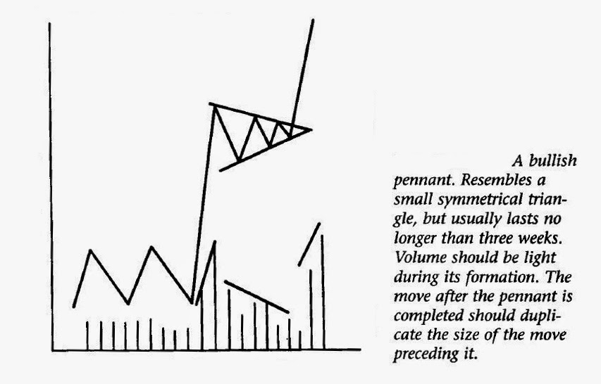
FLAGS AND PENNANTS

1. Flags and pennants are quite common, are similar in appearances, occur at about the same place in an existing trend, and have same characteristics.

2. They occur when market pauses briefly to catch breath after a steep move with heavy volume. when they are at the process of formation, the volume declines, then again bursts on a break out.

3. They rarely produce a trend reversal.


4. Flag is a parallelogram with a slop against the slope of the trend. 


5.  Pennant is a small symmetrical triangle.

6. The volume should decrease along the formation of the pattern. and the break out should be with heavier volume.

7. They take shorter time to form usually two to three weeks, down trend patterns are shorter in duration.

8. Both the patterns are formed in the mid point of a market trend.

WEDGE PATTERN


1.  Wedge pattern follows all the rules of the triangle pattern, except its implications and rules cited below. Please read also, the H&S pattern rules carefully.

2. The wedge pattern has a noticeable slant.

3. A down ward slopping wedge is a bullish pattern, and vice versa.

WEDGE REVERSAL PATTERN

Since a falling wedge is a bullish pattern, when it occurs at the end of a bear market, it might signal a trend reversal and vice versa.

RECTANGLE PATTERN


1. Rectangle is a trading range, a congestion area.

2. Rectangle pattern with 6 price swings, can be misinterpreted as a triple top reversal. Triple top reversal volume rules needs to be checked and the pattern ruled out, before confirming a rectangular pattern. Normally the rectangular patter resolves towards the trend direction. However, the direction of the heavier volume side determines to which side the rectangle break out finally will happen.

3. Minimum target rule follows the channel minimum target rules. Please read also, the H&S pattern rules carefully.


CONTINUATION HEAD AND SHOULDERS PATTERN


1. The continuation H& S pattern forms inverted to the reversal version in a continuing trends.

2. However the rules follow that of the rectangle formation.


Tuesday, 2 September 2014

Current Account Deficit Vs Fiscal Deficit, a simple explanation

I am starting with an extremely simple definition for the two.

Current Account Deficit

          It is the difference between the total exports and imports of the country. Current Account Deficit in a period happens when the imports in dollars crosses the exports for a country.

Fiscal Deficit 

          It is the difference between the total revenue ( Mainly from taxes ) of a country and the total expenditure ( Mainly public expenditures ) of a country. Fiscal deficit in a period happens when the expenditures crosses the revenue.

Saturday, 1 June 2013

Why profit is the highest when marginal cost curve crosses the marginal revenue curve ( Competitive firm model )

     The definitions and the characteristics for the various terms need to be referred to a standard text book. 

This blog will discuss only the reason for why the profit is maximized when Marginal cost curve crosses the Marginal revenue curve.

Abbrevations

MC=    Marginal Cost                                                     MR=   Marginal Revenue
ATC=  Average Total Costs                                           TC=     Total Costs
AVC=  Average Variable Costs                                     TR=     Total Revenue
AFC=  Average Fixed Costs                                          P=        Price; Q=    Quantity

Consider the following example

The table below gives the details of a factory producing a certain unit of a product.

Table 1


It is mentioned in a previous blog, why marginal cost crosses the Average cost curves at their lowest points,  and how the marginal cost, which is a change in cost, actually affects all the average costs.

EXPLANATION

Consider the following plots, plot 1 and plot 2 derived from the factory data in table 1.


Plot 1


Plot 2


The Total Cost is equal to Average Total Cost  multiplied by the quantity, and Total Revenue is equal to Average Total Revenue ( equal to price or MR for a competitive firm) multiplied by the quantity. Total Profit is the difference between the two.

In Plot 2, Total cost is drawn as an area which is equal to ATC multiplied by Quantity. And Total Revenue is drawn as an area which is equal to ATR multiplied by Quantity. Total profit is the Total Revenue area minus the Total cost area.

For example.

For a Quantity H, the TC=     area EYHF
                                 TR=      area DIHF
                                 Profit=  area DIYE.

For a Quantity G, the TC=     area ABGF
                                 TR=     area DCGF
                                 Loss=  area ABCD

CONFUSION

1.       In theory the profit has to be highest at a production output where the marginal cost crosses the marginal revenue, which is at point Z. whereas, it can be clearly seen that the Average total cost is lowest at point Y. And also, marginal cost is lower at point Y, which is lower than at point Z.

2.       At point W, the marginal cost is the lowest, much lower than the marginal revenue. But the production is at a significant loss at the same point.

CLEARING CONFUSION 1

Consider the following plots 3 and 4. Plot 3 plots the Total Revenue and Total costs. And plot 4, plots the difference of Total cost and Total Revenue ie the profit.


Plot 3


Plot 4


From plot 4 it is quite obvious that the maximum profit occurs at point Z ( where the MC crosses the MR). It is also observable from plot 3.

REASON    

The reason for this confusion is that, MC as defined previously is a change in cost. The difference between AVR( the straight line of $2) and the ATC curve gives us Average total profit(AVP), and it is quite clear that AVP is the highest at the point Y where ATC is the lowest. We get confused because we think that the profit should be highest when the AVP is the highest. But AVP is only an average. Increasing the production from point Y to point Z definitely reduces the AVP. But it increases the total profits. AVP is reduced because, each quantity  produced after point Y yeilds lesser profits, bringing down the average. But  the total profit gets increased albeit with decreased rate. Even when the Average Total Cost is at its lowest when the production reaches point Y (370 units), we can still squeeze in more profit per unit, by producing until the production reaches point Z (440 units) . Until then, each change in cost/ unit (MC) is still less than the price for which those units can be sold. The increase in total profits becomes zero only when the production reaches point Z. This is quite clear in the Plot 5.

 The difference between MR and MC is called Marginal profit, whereas, the difference between ATR and ATC is Average profit. In order to maximize the Total profit, we have to go on producing until the marginal profit is diminished to zero. Since Average profit is just an average, it might be still be positive for many more units of production even after the production crosses point Z. For more clarity refer to plot 5.

                                                                             Plot 5


In Plot 5, we can see that the average profit is maximum at point Y, which is self explanatory.

CLEARING CONFUSION 2

Marginal Cost, Marginal Revenue and Marginal Profit  are also the slopes of the Total Cost, Total Revenue and the Total profit curves respectively.

So in this case, when Marginal Cost is at the lowest, the Marginal Profit is at the maximum. But the factory is in loss. It just says that the slope of the Total cost curve is at the lowest and is about to change, and the slope of the Total profit curve is at the maximum and is about to change. At this point the Total cost is not the lowest, neither is the Total profit the highest. This is amply demonstrated in the plots 3,4 and 5.