Current Account Deficit Vs Fiscal Deficit, a simple explanation

I am starting with an extremely simple definition for the two.

Current Account Deficit

          It is the difference between the total exports and imports of the country. Current Account Deficit in a period happens when the imports in dollars crosses the exports for a country.

Fiscal Deficit 

          It is the difference between the total revenue ( Mainly from taxes ) of a country and the total expenditure ( Mainly public expenditures ) of a country. Fiscal deficit in a period happens when the expenditures crosses the revenue.

Why profit is the highest when marginal cost curve crosses the marginal revenue curve ( Competitive firm model )

     The definitions and the characteristics for the various terms need to be referred to a standard text book. 

This blog will discuss only the reason for why the profit is maximized when Marginal cost curve crosses the Marginal revenue curve.

Abbrevations

MC=    Marginal Cost                                                     MR=   Marginal Revenue

ATC=  Average Total Costs                                           TC=     Total Costs

AVC=  Average Variable Costs                                     TR=     Total Revenue

AFC=  Average Fixed Costs                                          P=        Price; Q=    Quantity

Consider the following example

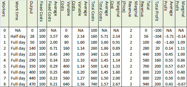
The table below gives the details of a factory producing a certain unit of a product.

Table 1

It is mentioned in a previous blog, why marginal cost crosses the Average cost curves at their lowest points,  and how the marginal cost, which is a change in cost, actually affects all the average costs.

EXPLANATION

Consider the following plots, plot 1 and plot 2 derived from the factory data in table 1.

Plot 1

Plot 2

The Total Cost is equal to Average Total Cost  multiplied by the quantity, and Total Revenue is equal to Average Total Revenue ( equal to price or MR for a competitive firm) multiplied by the quantity. Total Profit is the difference between the two.

In Plot 2, Total cost is drawn as an area which is equal to ATC multiplied by Quantity. And Total Revenue is drawn as an area which is equal to ATR multiplied by Quantity. Total profit is the Total Revenue area minus the Total cost area.

For example.

For a Quantity H, the TC=     area EYHF

                                 TR=      area DIHF

                                 Profit=  area DIYE.

For a Quantity G, the TC=     area ABGF

                                 TR=     area DCGF

                                 Loss=  area ABCD

CONFUSION

1.       In theory the profit has to be highest at a production output where the marginal cost crosses the marginal revenue, which is at point Z. whereas, it can be clearly seen that the Average total cost is lowest at point Y. And also, marginal cost is lower at point Y, which is lower than at point Z.

2.       At point W, the marginal cost is the lowest, much lower than the marginal revenue. But the production is at a significant loss at the same point.

CLEARING CONFUSION 1

Consider the following plots 3 and 4. Plot 3 plots the Total Revenue and Total costs. And plot 4, plots the difference of Total cost and Total Revenue ie the profit.

Plot 3

Plot 4

From plot 4 it is quite obvious that the maximum profit occurs at point Z ( where the MC crosses the MR). It is also observable from plot 3.

REASON    

The reason for this confusion is that, MC as defined previously is a change in cost. The difference between AVR( the straight line of $2) and the ATC curve gives us Average total profit(AVP), and it is quite clear that AVP is the highest at the point Y where ATC is the lowest. We get confused because we think that the profit should be highest when the AVP is the highest. But AVP is only an average. Increasing the production from point Y to point Z definitely reduces the AVP. But it increases the total profits. AVP is reduced because, each quantity  produced after point Y yeilds lesser profits, bringing down the average. But  the total profit gets increased albeit with decreased rate. Even when the Average Total Cost is at its lowest when the production reaches point Y (370 units), we can still squeeze in more profit per unit, by producing until the production reaches point Z (440 units) . Until then, each change in cost/ unit (MC) is still less than the price for which those units can be sold. The increase in total profits becomes zero only when the production reaches point Z. This is quite clear in the Plot 5.

 The difference between MR and MC is called Marginal profit, whereas, the difference between ATR and ATC is Average profit. In order to maximize the Total profit, we have to go on producing until the marginal profit is diminished to zero. Since Average profit is just an average, it might be still be positive for many more units of production even after the production crosses point Z. For more clarity refer to plot 5.

                                                                             Plot 5

In Plot 5, we can see that the average profit is maximum at point Y, which is self explanatory.

CLEARING CONFUSION 2

Marginal Cost, Marginal Revenue and Marginal Profit  are also the slopes of the Total Cost, Total Revenue and the Total profit curves respectively.

So in this case, when Marginal Cost is at the lowest, the Marginal Profit is at the maximum. But the factory is in loss. It just says that the slope of the Total cost curve is at the lowest and is about to change, and the slope of the Total profit curve is at the maximum and is about to change. At this point the Total cost is not the lowest, neither is the Total profit the highest. This is amply demonstrated in the plots 3,4 and 5.

Why the diminishing marginal utility curve has the same slope as the demand curve

Diminishing marginal utility states that, the marginal utility of a product diminishes with each unit of the product consumed.

This is because, the change in utility, when each unit of product is consumed, always decreases. ( refer to a standard text for more clarity)

ILLUSTRATION

Fig 1

Consider an example of ordering pizza, which costs one dollar a slice. If consuming the first slice gives 24 utils of utility, after eating the next one, the total utils increases to 36 utils. Refer to fig 1 for the complete pizza consumption.

You may notice that, had the price of a slice of pizza been $2, then the utility also reduces by half for each slice.

Fig 2

If we draw the total utility against number of slices consumed, the plot will look like fig 2

And therefore, if you plot the marginal utility in y axis and the number of unit consumed, in the x axis, you always get a curve with diminishing curve. This is called the diminishing marginal utility curve as illustrated in the fig 3 below.

Fig 3

If marginal utility of a product  is Mx at a price x, then Mx/x ie the marginal utility per dollar for that product should always be greater than that of any other alternative product, so that you may keep buying it.

So some one has to make you buy the same product  again and again, over every other alternative products, then the ratio Mx/x needs to be made constant, every time you consume the product.

Since marginal utility keeps on decreasing, while we consume the same product again and again, Mx decreases when more quantity is bought.

So inorder to keep Mx/x constant, the only way to do is the decrease the price, in the same ratio of decrease in Mx.

So the greater the price reduction, the more you will consume or demand. This is why the demand curve has the same slope as the marginal utility curve.

The demand curve is a plot produced, when the demand ( measured in quantity ) is plotted in x axis and the price plotted in the y axis.

The demand curve also has negative slope, ie the demand always diminishes when price is increased, keeping all other factors constant.

In the above pizza example, the demand curve would look like this

ILLUSTRATION

Product 1

let the marginal utility for a product be 100, 80, 60, 40, 20 for the first 5 pieces, and the price for the fifth piece is 20, then Mx/x for fifth piece is 1.

Product 2

If the marginal utility for another product be 100, 90, 70, 50, 40, and the price of the fifth piece is 20, then Mx/x for the fifth piece is 2.

If the seller has to make you take the fifth piece of the first product over that of the second product, then the marginal utility per dollar of the first product should be more than 2 ( marginal utility per dollar of the second product) . Ie the price of the fifth piece of the first product has to be reduced below 10 in order to make you buy the fifth piece of the first product over that of the second product.

This means that whenever you increase a price of a product, the demand diminishes.

Why Marginal cost curve crosses the Average Total Cost curve and the Average Variable Cost curve at their minimum point.

Refer to figure 1 given below.

                                                                        fig 1

All the data is taken from the chart in the blog on "Why the profit is maximised when the marginal cost curve crosses the marginal revenue curve"

Facts to consider

1. Average total cost curve is a plot of the average total costs for all the different quantities starting from zero production. The X axis is the quantity, and the Y axis is the ATC. This curve first slopes downward, then reaches a bottom and then slopes upward.

2. Average variable cost curve has the same characteristics of the ATC curve, but always stays below the ATC curve at all the points. The difference between the values of the curves is the fixed cost.

3. Since all the three curves has quantity in the x axis, all of them can be drawn together. The MC curve also first slopes downward, reaches a bottom and then starts sloping upward. The MC curve first crosses the AVC curve and then the ATC curve at their respective bottoms. Refer to a standard text on the problem.

TC       :                   Total cost
dTC     :                  Change in total cost
VC      :                   Variable cost
ATC    :                  Average total cost; AC is the average cost
dATC  :                  Change in ATC
AVC   :                  Average variable cost; VC is the variable cost
dAVC :                   Change in AVC
FC      :                   Fixed Cost.
Q        :                  Quantity.
dQ      :                  Change in Quantity.
MC     :                  Marginal cost.

MC    =                 dTC/dQ
TC     =                  VC + FC
dTC   =                  dVC+dFC

But since FC is the fixed cost and by definition does not change, dFC = 0

So dTC=dVC

So MC = dVC/dQ

            This means that marginal cost, which is the change in total cost per unit of quantity is actualy caused by the change in variable cost only. Now here the question is why the marginal cost curve crosses the Average total cost curve and the Average variable cost curve at their respective bottoms.

             Consider the average of height in a class. Whenever a new student joins, the average changes. If the height of the new student is the same as the present average, then the average does not change, if it is less the average decreases, if it is more the average increases. 

           
             Similarly, the marginal cost is the next new comer. Marginal cost is the next change in the cost (per unit). This next change, if it is more than the average, then the average will increase or vice versa.

             Since MC = dTC/dQ = dVC/ dQ. The new comer is same for both the averages TC and VC.

So, both the AVC and the ATC curve decreases and increases due to the new comer entry MC.

            Now, in the portion of the curves, where they have a downward slope, before they hit their bottoms, the marginal cost values are lesser than than the respective values of the average curves. So the lower MC values drags the averages down. Now when the MC curve, which hits the bottom of its own, slopes upward and first crosses the AVC curve. At the crossing point MC value = AVC value. And after that the MC values drags the AVC curve upwards. This is also what happens to the ATC curve.

            Note that MC is the new comer for both the the averages as we proved earlier.

 

TAX ASSETS, LIABILITIES AND REVENUE ACCOUNTS

       There are two situations in which usually some special accounts are used for recording the consequent tax effects.

1. Loss carry backs and loss carry forwards.

2. Temporary miss match in the calculation of taxable income between the methods acceptable under GAAP and tax department rules. Special accounts are not used for permanent differences.

The various special accounts used are

a. Tax refund Receivable.  (asset account)

b.  Tax benefit from carry back. (revenue account)

c.  Tax benefit from carry forward. (revenue account)

d.  Differed tax asset. (asset account)

e. Differed tax liability.(liability account)

  The first three accounts are used in situation 1 only. The differed tax asset account is used in both the situations. Differed liability account is used only in situation 2.

Situation 1. LOSS CARRY BACK AND CARRY FORWARD

   

LOSS CARRY BACK

   In some countries, a loss in an year is allowed to be carried back. The extent of the carry back depends upon the accounting rules. This means that the net loss can be absorbed into the net incomes of the previous years, which in turn reduces these net incomes. This makes the tax payed on these previous incomes, over paid. This over paid cash can be claimed back from the tax department in cash.

eg: Suppose the net incomes of the previous 2 years for a company totals $400000 and the net loss in the current year amounts to $600000. If the tax rule is the net loss can be carried back only for 2 previous years, and tax rate is 30%

tax reclaimable = $400000*30%=$120000. 

The entry is

Tax refund receivable                      120000

Tax benefit from carry back                                  120000

LOSS CARRY FORWARD

    If the previous example is examined, it can be seen that the net income total for the previous 2 years of $400000 is inadequate for completely absorbing the net loss of $600000. In order to get a tax relief on the balance of $200000 net loss, the tax rules of some countries allow this loss to be carried forward to as far as 20 years and only if some conditions are met.

The total tax relief that can be claimed in the future, which is calculated using an estimated future tax rate, is carried in the balance sheet as an intangible asset called the differed tax asset. This asset account is cumulative in nature.

Here the net loss carry forward = $200000

if the estimated future tax rate is 30%,

then the differed tax asset=           $60000

   suppose in the previous example, the net income for the next year is $300000, and if the tax rate is 30%, and if all conditions necessary are met, then

The total tax payable =$300000*30%=$90000

this tax payable can be offset with the differed tax asset of $60000

The entry is

Income tax expense             90000
Differed tax asset                                    60000
Income tax payable                                30000

Here, though the income tax expense is recorded completely, the tax payment is done only after subtracting the balance in the differed tax asset account.

Had the net income for the next year was $ 100000, the income tax expense would have been $30000, and the entry would have been

income tax expense             30000
differed tax asset                                   30000

Since the income tax expense is less than the accumulated differed tax asset, no cash had to be paid.

If we analyse the above examples the differed tax liability is never used in situation 1.

Situation 2. TEMPORARY MIS MATCH IN TAXABLE INCOME CALCULATION.

In most countries, the accounting for tax under GAAP rules, varies widely with the accounting rules of the tax department. This results in many type of temporary or permanent differences between the taxable incomes calculated under these two rules.

SITUATION 1.

This happens when income earned in a year but not received by the year end is added in the net income under GAAP but not added in the net taxable income under tax rules. This makes the net income taxable, calculated under the GAAP rules greater than that under the tax rules. So are the consequent taxes.

SITUATION 2.

This happens when income received in a year but not earned in the same year, is added in the net taxable income under tax rules, but is not added in the net taxable income under GAAP rules. This makes the former greater than the later. So are the consequent taxes.

SITUATION 3.

Thus happens due to different estimates used for future income and expenses.


SITUATION 4.

Due to tax departments not recognizing some income or expenses for tax purposes. These includes life insurance premiums, tax free bond interests etc which are admitted in calculating the taxable income under GAAP but not under the tax rules.

TEMPORARY DIFFERENCES

The first three situations are mostly temporary differences, because they will ultimately self correct.

An example for situation 1. 

An expense accrued in this year under GAAP may not be admitted for calculating the taxable income until payed for,under the tax rules. This causes net income calculated under GAAP, greater than that which is calculated according to tax rules. So will be the consequent taxes. But this decrease is compensated when the expense is finally payed in cash in a later year. This causes a liability called differed tax liability- a liability to pay the tax in cash in the future.

An example for situation 2.

An unearned revenue which is a payment in cash in advance, may be allowed to be added to the net taxable income under tax rules, but not admitted as an income under GAAP rules. This causes the taxable income under the tax rules to be more than that of which is calculated under GAAP rules. And so are the consequent taxes. And the tax is over paid in the current year though not required under the GAAP rules. This over payment creates a prepaid asset called a differed tax asset.

An example for situation 3.

If straight line method of depreciation is used under GAAP while accelerated method is used under tax purposes for the same life for an asset, then the net income for the initial years under GAAP (and subsequent tax payed) will be more than that calculated by tax rules. But in the later years the depreciation expense will be less under accelerated method and consequently, the net income (and the consequent tax) will be less under GAAP when compared to that under the tax rules, which causes the self correction.

DIFFERED TAX LIABILITY IN TEMPORARY DIFFERENCES (situation 1)

Suppose net taxable income under GAAP is $110000, and under tax department rules is $100000, if tax rate is 30% and we assume that the difference of $10000 is temporary.

for calculation purposes, we divide the figures into regular income and the temporary difference.

regular income=$100000;
temporary difference=$10000;

regular tax component=$30000
temporary tax component=$3000

This temporary tax component, which will have to be paid in the future(as shown in the entry given below) is carried in the balance sheet as a liability called the differed tax liability. This is because, this component is a payment which we have to make in the future, which we have not made now because we do not need to pay now according to the tax rules. This is an accrued liability.

The entry is

Income tax expense            33000
Differed tax liability                                  3000
Income tax payable                                 30000

Note that the differed tax liability account is also a cumulative account.

Suppose next year the net income under GAAP is $100000, and under dept rules is $110000

Income tax expense           30000
Differed tax liability             3000
Income tax payable                                 33000

Thus the tax difference which had to be paid in the next year, which was recorded as a differed tax liability, is paid in the next year from the same differed tax liability account set up for the same purpose.

DIFFERED TAX ASSET IN TEMPORARY DIFFERENCES (situation 2)


Suppose net taxable income under GAAP is $100000, and under tax department rules is $110000, if tax rate is 30% and we assume that the difference of $10000 is temporary.

for calculation purposes, we divide the figures into regular income and the temporary difference.

regular income=$100000;
temporary difference=$10000;

regular tax component=$30000
temporary tax component=$3000

This temporary tax component, which is pre paid (as shown in the entry given below) in the current year  is carried in the balance sheet as an asset called the differed tax asset. This is because, this component is a payment which we need not pay according to the GAAP rules, which we have already prepaid as required by the tax rules. This is a prepaid asset.

The entry is

 income tax expense            30000
differed tax liability              3000
income tax payable                                 33000

Note that the differed tax asset account is also a cumulative account.

Suppose next year the net income under GAAP is $110000, and under dept rules is $100000

income tax expense             33000
differed tax asst                                         3000
income tax payable                                  30000

COMPOUND ENTRY IN TEMPORARY ACCOUNTS

Consider the following situation

A company has a net taxable income under GAAP of $110000. The taxable income under tax rules is $108000. And we also find that $10000 in the GAAP income, is income earned but not received in cash and $8000 in the tax rules income is income received but not yet earned, then

Here before making the entries a preliminary calculation also has to be made

Regular income=$100000; tax =$30000
Income earned but not received in cash=$10000; tax payable=$3000
Income received in cash but not earned=$8000; tax prepaid=$2400
Tax payable according to tax rules= $32400 (30% of $108000)

The entry will be


Income tax expense     33000
Differed tax asset          2400
Differed tax liability                     3000
Income tax payable                      32400

There are many different rules for recording temporary differences for various situations other than those mentioned above. Some of these situations are mentioned below.

1. The tax rate gets changed for future years and is known in the current year.

2. The tax rate is expected to change for future years but has not yet changed.

3. Accrued tax liabilities are paid over a multiple number of years.

4. Prepaid tax assets are compensated over a multiple number of years.

5. Any combination of the above.

The accounting for these are beyond the scope of this post, and an be consulted in an intermediate accounting textbook.

Accrued liabilities/assets vs unearned revenue/prepaid assets

  For the definitions and accounting for these accounts, the articles posted before this date on these topics needs to be reviewed

COMPARISON

1. Accrued liability is an opposite counterpart of the accrued assets account. And the unearned revenue account is the opposite counterpart of the prepaid expenses account.

Accrued liability eg:

                     Expense     xxx
                     Accounts payable               xxx
(Cash payment is postponed, but expenses recorded)

When the cash is finally paid, the liability is reduced.

                     Accounts payable      xxx
                    Cash                                         xxx

Accrued Assets eg:

                      Accounts receivable   xxx
                      Revenue                                    xxx
(Cash is not received, but revenue is recognized)

When the cash is finally received, the asset is reduced.

                    Cash         xxx
                    Accounts receivable               xxx

Unearned revenue eg:

                      Cash       xxx
                      Extended Warranty Payable             xxx                                  
OR

                      Cash       xxx
                      Advance Received            xxx

Unearned revenue is a liability. Though cash is received, the revenue is not recognized until the task required to earn the revenue is not complete. Since  this cannot be brought as a part of income untill it is recognized, it is capitalized as a liability in the balance sheet, and is amortised as an when the task gets complete.

                      Advance Recieved       xxx
                       Sale                                             xxx

                     Extended Warranty Payable      xxx
                      Extended Warranty Revenue                   xxx

But unfortunately if we cannot complete the task or in case an extended warranty claim actually has to be paid back, then this revenue is reversed with an expense.

                     Advance Recieved    xxx
                     Cash                                             xxx

                     Extended Warranty Payable      xxx
                     Cash                                                           xxx


Prepaid expense     eg:

                       Rent for 3yrs paid        xxx
                       Cash                                               xxx

We cannot recognise the expense for future years in the current year. But we have already paid for future years. So this is an asset (because technically we can get back the money if the expected task is not completed) and is capitalised as such in the balance sheet. This is also amortised as and when the task for which we have paid in advance gets completed

                      Rent expense for current year    yyy
                      Rent for 3yrs paid                                        yyy

And if we do not want the task to get completed and gets  our money back,
                      Cash               xxx
                       Rent for 3yrs paid                                        xxx
                 

2. Accrued liability and unearned revenue are both liability accounts  whereas accrued assets and prepaid expenses are both asset accounts.

3. Accrued liability and accrued assets debits and credits an expense and a revenue account respectively, whereas unearned revenue and prepaid expenses debits and credits a cash account respectively.

4. Accrued liability and accrued asset account are reduced when the cash is paid and received respectively, whereas Unearned revenue and prepaid assets are reduced when the revenue and the expenses are finally recognised.

The unique thing about Contingent Liabilities

            A contingent liability an accrued liability. As with an accrued liability,which is a non cash liability,  no cash is taken from anybody to create a contingent liability. Instead we fear we may have to pay for something, soon, and thus create a liability by recording an expense.

Let us examine some examples.

         A typical example is the accounting of warranty. When we sell a product, we have to give warranty. Since we cannot charge warranty fees from the customers, we charge it indirectly while the product is sold. The entry is

  cash                                            1000000

  est warranty exp (3yrs)                200000

  est warranty liability                                          200000

  sales                                                                  1000000

Here the product is sold for 1200000, and the estimated warranty expense 200000 is recorded and a consequent liability is capitalized in the balance sheet. As we know, when an expense is made, the retained earning is reduced by the same amount. So 200000 is reduced from the capital to create a liability of the same amount. Now when the warranty is claimed by the customer for say 50000, that expense which is paid in cash, reduces the liability.

  est warranty liability                     50000

 cash                                                                     50000

If this is the only amount claimed during the entire warranty period of 3 years, we remove the unclaimed liability by adding it back to the retained earnings (capital) through a revenue entry

 est warranty liability                     150000

 warranty revenue                                                1500000         

Another example is that of a probable and estimable lawsuit settlement. We create a contigent liability called lawsuit settlement liability.

  lawsuit settlement exp               xxxxx

  lawsuit settlement liability                                xxxxx

When the settlement actually happens

  lawsuit liability                            xxxxx

  cash                                                                   xxxxx

for eg:

  cash                                  1000000

  est warranty exp                200000

  est warranty liability                              200000

  sales                                                       1000000

  est warranty liability         4000

  cash                                                            4000 (when claimed)

UNIQUENESS

The uniqueness of contingent liabilities is that they don't have an opposite called contingent asset. Yes, there are certain short lived asset additions made which goes into gain section in the income statement like the following entry

Investment-Securities.                             xxx
Gain on appreciation of securities.                             xxx
This is done  when an investment in security is declared as a dividend; the security in question is revalued to its fair market value. But the nature of Investment-Securities is short term. This account gets removed from the balance sheet once the said dividend is paid.

 We do not create a revenue by dreaming that we will gain/win an income, creating a contingent asset.

For example

 Lawsuit receivable        100000000
Lawsuit win revenue                             100000000    

As you can see this is as absurd as it seems.